Looking into the Future
Modeling the Outputs of the Multivariable Process Map
(Post 10)
In the previous three blog entries, we have discussed the basic construct of process and theory around multivariable process maps. Each operation in a multivariable process map has labor, a cost, and in some cases, a yield. In this chapter we are going to use a simple example process to introduce how product development, process and manufacturing development, operations, and supply chain can use the multivariable process map to start to understand how decisions are shaping the overall cost and required resources to realize your hard-tech product.
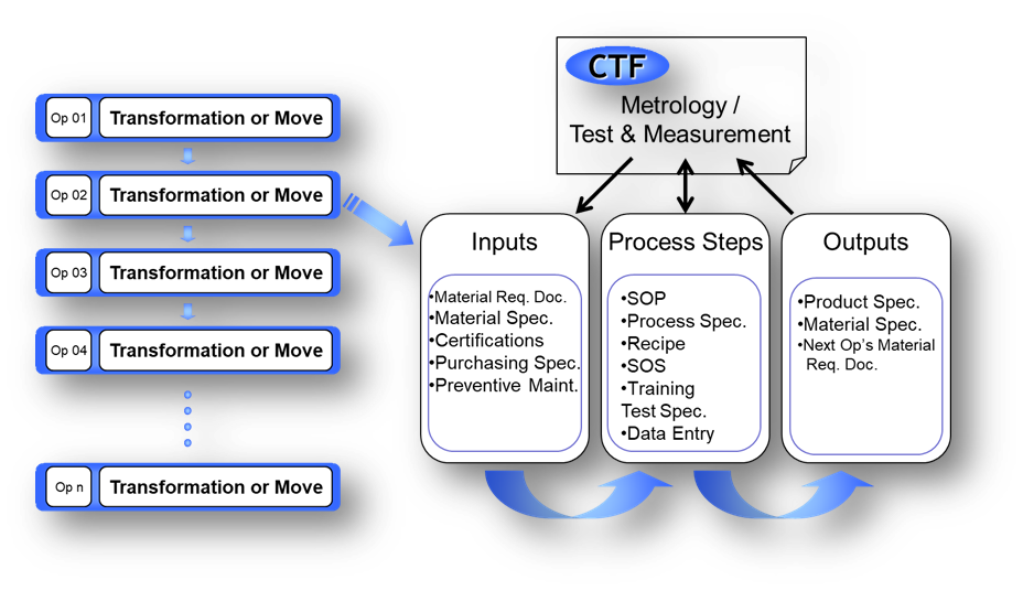
Here is the basic process map construct for reference.
A sample process for a sample product
As an illustration of these techniques and principles, I have created a process that we can refer to. (Eagle eyed blog fans may recognize this sample; it was attached to the previous chapters as a liked Excel Process Map to download and edit.) The idea was to make it simple, but realistic enough for scenario modeling and problem solving.
The 10-step process creates a fictional product, a Low Frequency Acoustic Absorber that is intended to improve the performance of micro-subsonic detectors, for home seismographs. Our “research” and the development of our Marketing and Product Requirements Document determined that low-cost detectors could be used if there was better absorption of sound in these frequencies. Californians and residents of other earthquake-prone areas have demanded this low-cost in-home capability for years, allowing them to quickly determine if evacuation is needed, and to configure their survival packs depending on the severity of the event. Micro-subsonic detector system providers are looking for new markets, but without our product, they cannot meet the selling price point with their more expensive detector. With our technology, they can leverage older technology.
The key technology driving this product is the sensor that makes up the fictional low frequency acoustic absorber, made up of a small, printed circuit board. They will be produced on a wafer “substrate” that holds 50 of our devices, laid out in a 5x10 matrix. Later in the process, the wafer will be “diced” or cut into pieces to make 50 individual units.
Micro-subsonic detector at wafer and device levels
The basic steps for production will be to prepare and clean the substrate, to carefully position the microfilm for “printing” and lamination, dispense a polymer adhesive material, cure, test, and dice. As in any PCB or microelectronic assembly process, each of these steps has a very particular set of parameters that can greatly influence the outcome and success of the final product, so precision is of paramount importance.
Market Demands for our fictional product
Our customer projects the following demand and target pricing for the product:
Quantities and Demand per Period and Target Device Cost at Volume:
Our constraints are:
The finished Sensor Devices per current substrate size: 50 absorbers.
The target cost is $4.50 per Sensor based on marketing and systems’ requirements, and the actual starting cost based on preproduction values is $16.50 per Sensor.
For the system to be profitable, the breakeven cost is $10.00 per Sensor, the team is committing to that goal by Q1-2024.
Labor is fixed regardless of substrate size, and substrate cost increases 0.25 times for every doubling of area.
Q3-FY2023 Starting Multivariable Process Map
What do we get for our Multivariable Process Mapping efforts?
Coming up with, reviewing and revising, and verifying the information in our Process Map is a substantial effort. But lots of useful benefits roll out of the model. The first thing we get is a quantitative visualization of our process and how our design could be built. In manufacturing lingo, this is a routing. The second thing we get is an estimation of the materials used. In design and manufacturing lingo, this is Bill of Materials or BOM.
We can also extract critical information around the cost of materials and supplies, Costed Bill of Materials. The total labor involves manufacturing a device and the total time required to manufacture as device, or the Cycle Time. We can also determine the total cost for equipment.
Let’s take a look at the outputs from our model for Q3-2023:
From a commercialization perspective, this may be your first view of critical factors that will be the foundation for manufacturing your product. You now know that you need ~40 minutes (0.67 hours) to manufacture a substrate. Your theoretical cycle time is ~180 minutes (3.00 hours).
Scaling Up
Over time, we expect volume will go up and price will go down. Even at this early stage, we can project the timeline for the expected volume changes and the target pricing, but we need to plan what technical or material improvements will lead to those cost reductions. Price breaks from material suppliers as volume goes up and yield improvements as our manufacturing process stabilizes will be contributing factors, but to make further cost reductions, we need to look to what other improvements can be made, such as automation.
Target Device Cost at Volume:
If you download the full spreadsheet of our sample Process Map, you will notice worksheets for these future quarters. Click the tabs to see the Process Maps as they change over time (highlighted in Yellow), allowing us to see these detailed cost and yield projections for the future.
Understanding yield
In a subsequent entry, we will spend some time on the finite capacity and planning. But for now, let’s concentrate on yield and its huge impact on labor and material cost.
Often when training new operations teams at startups, the team mindset is optimistic. Usually after a few workshops and sessions we can come to agreement on the basic labor and materials. Usually, individual operations can be demonstrated successfully. But when I asked if the operations can be performed in the proposed sequence, silence ensues. Crickets. I usually push and ask what happens, almost always they describe a situation where no product makes it through all the processes, or the product that makes its way through fails for some basic parameter or specification. Or I get the answer that “Bill the Technician” can get stuff to pass if it’s a Tuesday morning with a waning moon, but no one else can.
This is yield. Yield can be called many things. For example, in traditional quality theory, yield is related to Percent Defective (p’), whereas Yield is equal to 1-p’. If you have 10% defective, you have 90% yield. In the world of traditional Statistical Process Control, the factor CpK or process capability coefficient can be related to Z-Scores (Normal Distribution) and Part per Million (ppm), both which represent p’.
In rolled yield modeling, or single piece flow modeling, which is common in Hard-Tech, time is constant. What this means is when time is consumed, you lose it forever. In the extreme situation above with Bill the Technician, nothing is passing the quality inspection required. In a more realistic situation and usually the outcome of the additional workshops, we learn that there is actual one or two operations or tests that cause the huge yield impact. Usually, we find a process that lacks process capability, the design lacks performance margin, and a test station that lacks repeatability and reproducibility.
Remember we constrained this discussion saying time is constant. Why? We want to understand the theoretical model and the actual. If you consider our absorbers, our Rolled Yield is 75%. In real world that means we need start 1.33 units to get one successful unit. But we can’t start with 1.33 units; we need to start with 2, and therefore need twice as many machines, labor, and materials to meet the one unit in the same amount of time.
What? Time is constant, remember. And you need to produce one unit.
In production volume (quantities), it’s not as drastic. If we were producing 100 units, we could start with 133. That’s still not great, but it’s fewer than 200! But understanding yield – preferably, before volume production begins – is a critical way to determine production success.
Full Arc Posts Table of Contents
Post 4 - Defining Product Requirements
Post 5 - Exploring the Product Life Cycle
Post 6 - Understanding Risks in Real Time
Post 7 - A Deep Dive on Process Modeling
Post 10 - Looking into the Future
Post 11 - Keeping an Eye on The Next Generation
Post 12 - Product Platforms


